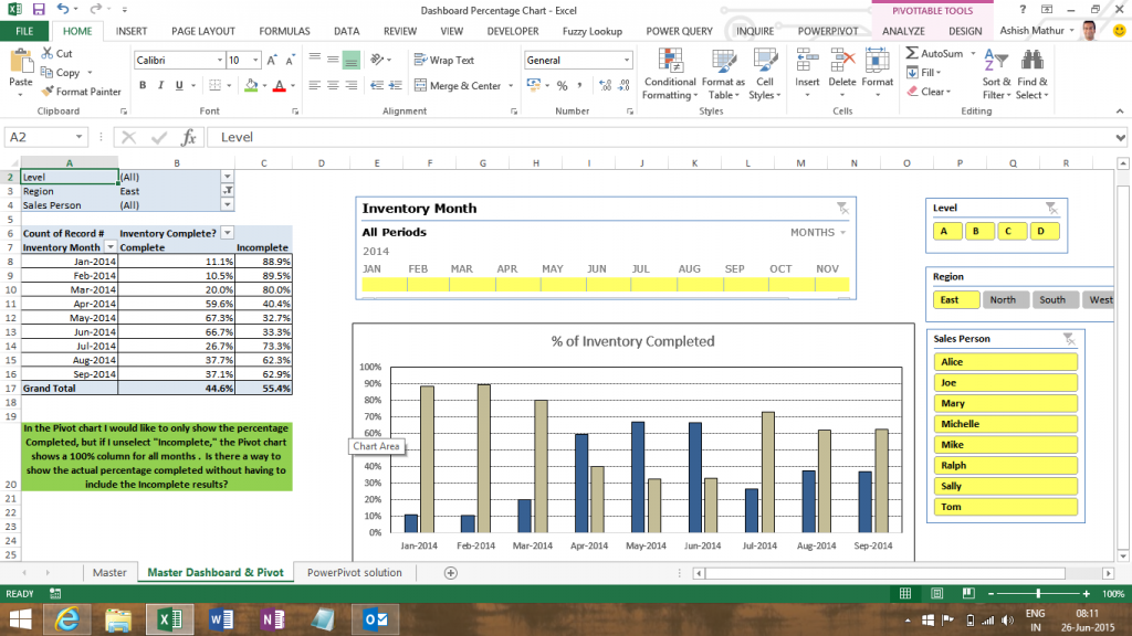
Here is a dashboard created with a Pivot Table, a Pivot chart and slicers (Click to enlarge image). In the Pivot Table, the % have been computed using “% of row total”.
The Pivot chart shows two columns per month – one for complete and the other for incomplete. The objective is to show only the Complete column per month in the Pivot chart. If one filters the Pivot Table only on Complete, then the Pivot chart shows an unexpected result – each column will go upto 100%. This happens because all calculations in a Pivot Table happen only on the visible cells. Once the Incomplete column is hidden, the “% of row total” calculation will return 100% which in turn reflects in the Pivot chart.
I have resolved this problem with the help of the PowerPivot. You may refer to my solution in this workbook.


Workaround to the problem of creating a Pivot chart after using “% of row total” calculation in a Pivot Table
{ 0 Comments }